Overview
This vignette demonstrates how to compare estimates from a validation run (using a subset of data) against estimates from a full data run. This is useful for assessing how well the model performs when some data is held out.
Data
The package includes example eta estimates from both a full data run and a validation run:
head(eta_example)
#> # A tibble: 6 × 6
#>   iso    year   eta  draw cluster                      subcluster
#>   <chr> <int> <dbl> <int> <chr>                        <chr>
#> 1 AFG    2023 0.335     1 North Africa and Middle East North Africa and Middle …
#> 2 AFG    2023 0.306     2 North Africa and Middle East North Africa and Middle …
#> 3 AFG    2023 0.339     3 North Africa and Middle East North Africa and Middle …
#> 4 AFG    2023 0.324     4 North Africa and Middle East North Africa and Middle …
#> 5 AFG    2023 0.290     5 North Africa and Middle East North Africa and Middle …
#> 6 AFG    2023 0.304     6 North Africa and Middle East North Africa and Middle …
head(eta_val_example)
#> # A tibble: 6 × 6
#>   iso    year   eta  draw cluster                      subcluster
#>   <chr> <int> <dbl> <int> <chr>                        <chr>
#> 1 AFG    2023 0.188     1 North Africa and Middle East North Africa and Middle …
#> 2 AFG    2023 0.535     2 North Africa and Middle East North Africa and Middle …
#> 3 AFG    2023 0.293     3 North Africa and Middle East North Africa and Middle …
#> 4 AFG    2023 0.320     4 North Africa and Middle East North Africa and Middle …
#> 5 AFG    2023 0.174     5 North Africa and Middle East North Africa and Middle …
#> 6 AFG    2023 0.334     6 North Africa and Middle East North Africa and Middle …
Summary Statistics
Use summarize_eta_all() to compute error metrics and
coverage statistics:
val_summary <- summarize_eta_all(
  res_val = eta_val_example,
  res_all = eta_example,
  year_select = 2023
)

knitr::kable(val_summary, digits = 3)| ncountries | ME | MAE | MeanE | MeanAE | Coverage | Prop_above_CI | Prop_below_CI |
|---|---|---|---|---|---|---|---|
| 47 | -0.006 | 0.033 | -0.005 | 0.048 | 0.924 | 0.029 | 0.047 |
Interpretation
- ME (Median Error): Median of (full data estimate - validation estimate)
- MAE (Median Absolute Error): Median of absolute errors
- MeanE / MeanAE: Mean versions of the above
- Coverage: Proportion of full data draws that fall within the validation 95% CI
- Prop_above_CI / Prop_below_CI: Proportion of full data draws above/below the validation CI
Good validation performance is indicated by:
Error metrics close to zero
Coverage at or above 0.95 (the nominal level)
Regional Comparison
You can subset the data to compare validation performance across regions:
# Sub-Saharan Africa only
val_summary_ssa <- summarize_eta_all(
  res_val = eta_val_example %>% filter(cluster == "Sub-Saharan Africa"),
  res_all = eta_example %>% filter(cluster == "Sub-Saharan Africa"),
  year_select = 2023
)

knitr::kable(val_summary_ssa, digits = 3, caption = "Sub-Saharan Africa")| ncountries | ME | MAE | MeanE | MeanAE | Coverage | Prop_above_CI | Prop_below_CI |
|---|---|---|---|---|---|---|---|
| 25 | -0.001 | 0.042 | 0.003 | 0.063 | 0.913 | 0.046 | 0.041 |
# Other regions
val_summary_other <- summarize_eta_all(
  res_val = eta_val_example %>% filter(cluster != "Sub-Saharan Africa"),
  res_all = eta_example %>% filter(cluster != "Sub-Saharan Africa"),
  year_select = 2023
)

knitr::kable(val_summary_other, digits = 3, caption = "Other regions")| ncountries | ME | MAE | MeanE | MeanAE | Coverage | Prop_above_CI | Prop_below_CI |
|---|---|---|---|---|---|---|---|
| 22 | -0.013 | 0.019 | -0.014 | 0.03 | 0.937 | 0.01 | 0.053 |
Visualizing Errors
We can create a boxplot to visualize the distribution of errors by region:
year_select <- 2023

# Calculate errors per country
errors_df <- eta_val_example %>%
  filter(year == year_select) %>%
  group_by(iso) %>%
  summarise(
    median_val = median(eta),
    cluster = first(cluster),
    .groups = "drop"
  ) %>%
  left_join(
    eta_example %>%
      filter(year == year_select) %>%
      group_by(iso) %>%
      summarise(median_all = median(eta), .groups = "drop"),
    by = "iso"
  ) %>%
  mutate(
    error = median_all - median_val,
    region = ifelse(cluster == "Sub-Saharan Africa", "Sub-Saharan Africa", "Other")
  )

head(errors_df)
#> # A tibble: 6 × 6
#>   iso   median_val cluster                            median_all    error region
#>   <chr>      <dbl> <chr>                                   <dbl>    <dbl> <chr>
#> 1 AFG        0.270 North Africa and Middle East            0.327  0.0569  Other
#> 2 ARG        0.934 LAC                                     0.918 -0.0159  Other
#> 3 BEN        0.542 Sub-Saharan Africa                      0.541 -0.00105 Sub-S…
#> 4 BFA        0.472 Sub-Saharan Africa                      0.747  0.275   Sub-S…
#> 5 BGD        0.621 South Asia, Southeast Asia, and O…      0.565 -0.0560  Other
#> 6 BLR        0.992 Central Europe, Eastern Europe, a…      0.998  0.00665 Other
ggplot(errors_df, aes(x = region, y = error, fill = region)) +
  geom_boxplot(alpha = 0.7) +
  geom_hline(yintercept = 0, linetype = "dashed", color = "red") +
  scale_fill_manual(values = c("Sub-Saharan Africa" = "forestgreen", "Other" = "steelblue")) +
  labs(
    title = sprintf("Validation Errors by Region (Year %d)", year_select),
    x = "",
    y = "Error (Full data - Validation)"
  ) +
  theme_bw() +
  theme(legend.position = "none")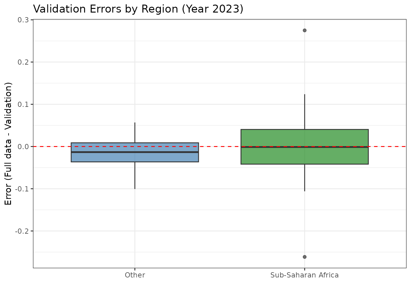
Errors centered around zero (the red dashed line) indicate good validation performance. Systematic deviations may suggest issues.