Smoothing Model Checks • bayescoveragemodelchecks

library(bayescoveragemodelchecks)
library(dplyr)
library(ggplot2)

Overview

This vignette demonstrates how to use the bayescoveragemodelchecks package to detect systematic patterns in residuals (or innovation terms) from Bayesian transition models.

Approach

For each posterior sample $j = 1, 2, \ldots, J$ , we have a set of residuals $(z_1^{(j)}, \ldots, z_n^{(j)})$ , with associated standard deviations $(s_1^{(j)}, \ldots, s_n^{(j)})$ , and predictor values $(x_1, \ldots, x_n)$ (e.g., coverage level or year).

For each posterior sample $j$ , we fit a weighted smoothing spline $f(x)^{(j)}$ that captures the relationship between residuals $z$ and predictor $x$ , accounting for the standard deviation associated with each residual.

We summarize the results by calculating the posterior probability that the fitted smoother deviates from zero at any value of $x$ :

$\text{Evidence} = 2 \cdot \min\{P(f(x) > 0), P(f(x) < 0)\}$

Values close to 0 indicate strong evidence of a systematic trend
Values close to 1 indicate no evidence of trend (residuals centered around zero)
We suggest that values below 0.1 should be investigated.

Example 1: No systematic trend

We’ll use the example residuals included in the package:

data("residuals_example")
head(residuals_example)
#> # A tibble: 6 × 17
#>   obs_index         y y_prop held_out iso    year cluster subcluster name_region
#>       <int> <dbl[1d]> <dbl[> <lgl>    <chr> <dbl> <chr>   <chr>      <chr>      
#> 1         1     -1.05  0.146 FALSE    AFG    2011 North … North Afr… Asia       
#> 2         1     -1.05  0.146 FALSE    AFG    2011 North … North Afr… Asia       
#> 3         1     -1.05  0.146 FALSE    AFG    2011 North … North Afr… Asia       
#> 4         1     -1.05  0.146 FALSE    AFG    2011 North … North Afr… Asia       
#> 5         1     -1.05  0.146 FALSE    AFG    2011 North … North Afr… Asia       
#> 6         1     -1.05  0.146 FALSE    AFG    2011 North … North Afr… Asia       
#> # ℹ 8 more variables: data_series_type <chr>, draw <int>, yhat <dbl>,
#> #   sd_y <dbl>, level <dbl>, level_prop <dbl>, sd_y_prop <dbl>,
#> #   residual <dbl[1d]>

Run the residual smoothing analysis:

results <- residual_model_check(

  res_data = residuals_example,
  predictor = "level_prop"
)

Visualize smoothing fits

The plot below shows the smoothing curves across all posterior draws:

Grey lines: individual smoothing curves for each posterior draw
Red dashed line: median fit
Red ribbon: 95% credible interval

plot_smoothing_fits(results,
                     x_lab = "Coverage level",
                      y_lab = "Smoothed residual",
                            title = "Residual smoothing fits",
                            subtitle = "Smoothing fit (grey), median (red line), 95% CI (area)")

Evidence metric

The evidence metric shows the probability that the residual trend does not deviate from zero:

plot_smoothing_summary(results, x_lab = "Coverage level")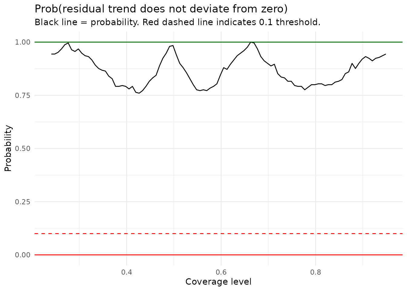

Summary

min_evidence <- summarize_smoothing_results(results, verbose = TRUE)
#> === Analysis ===
#> Prob(residual trend does NOT deviate from zero): 0.760
#> Interpretation: low values indicate strong evidence of systematic trend;
#>                 high values indicate no strong evidence of trend.

The minimum evidence value is 0.76. Since this is well above 0.1, we conclude there is little evidence of systematic trends in the residuals.

Example 2: With systematic trend

To demonstrate detection of a trend, we artificially add a systematic pattern to the residuals:

residuals_with_trend <- residuals_example
residuals_with_trend$residual <- residuals_with_trend$residual +
  0.1 * (residuals_with_trend$level_prop - 0.5)

results_trend <- residual_model_check(
  res_data = residuals_with_trend,
  predictor = "level_prop"
)

plot_smoothing_fits(results_trend, 
                    x_lab = "Coverage level",
                      y_lab = "Smoothed residual",
                            title = "Residual smoothing fits",
                            subtitle = "Smoothing fit (grey), median (red line), 95% CI (area)")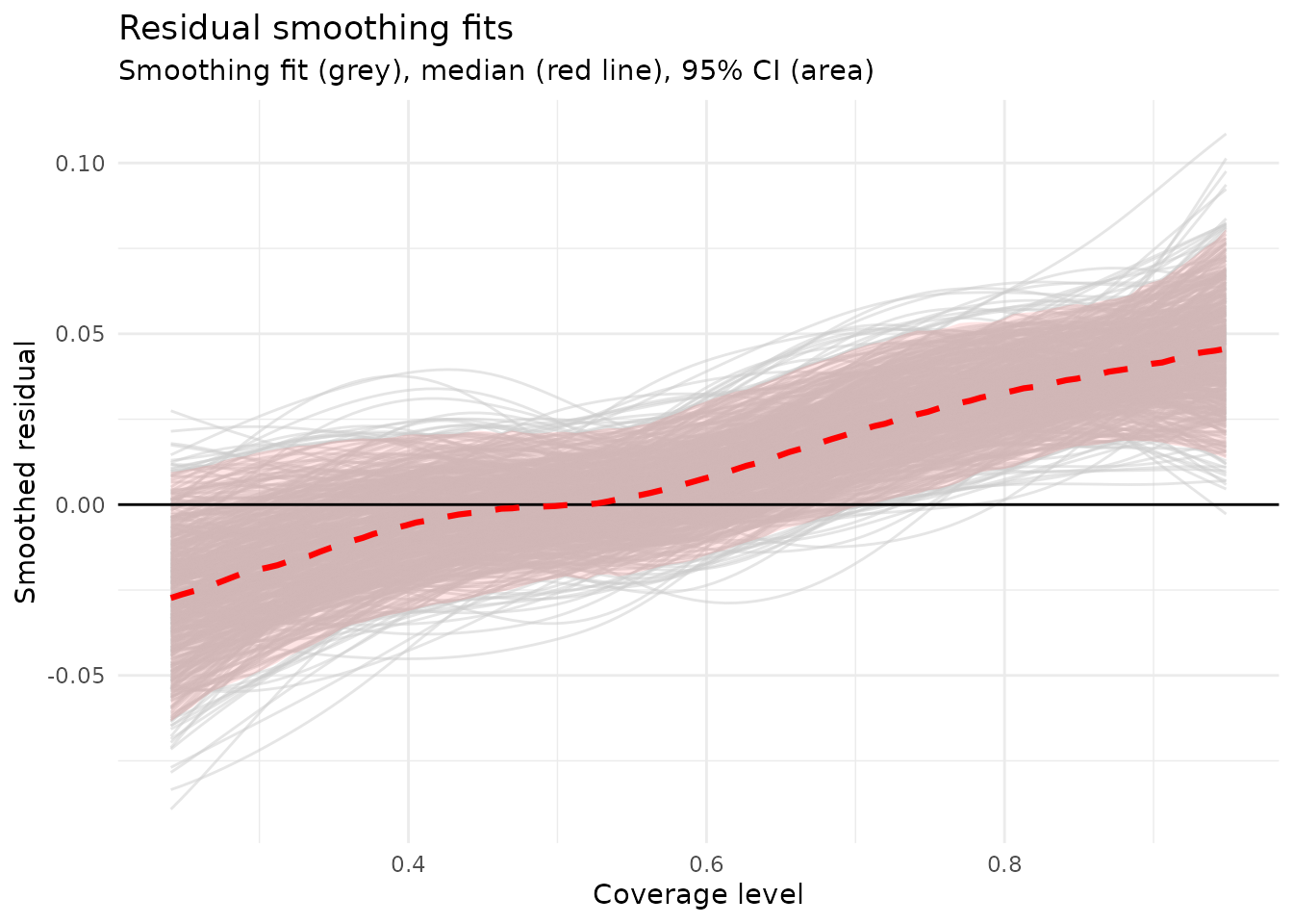

plot_smoothing_summary(results_trend, x_lab = "Coverage level")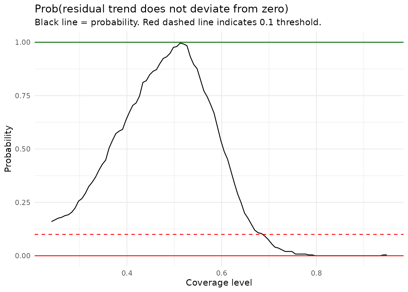

min_evidence_trend <- summarize_smoothing_results(results_trend, verbose = TRUE)
#> === Analysis ===
#> Prob(residual trend does NOT deviate from zero): 0.000
#> Interpretation: low values indicate strong evidence of systematic trend;
#>                 high values indicate no strong evidence of trend.

The minimum evidence value is now 0. Since this is below 0.1, we conclude there is evidence of a systematic trend in the residuals, suggesting potential model misfit.

Summary table for examples 1 and 2

summary_df <- data.frame(
  Analysis = c("Original residuals", "Residuals with trend"),
  Min_Evidence = c(min_evidence, min_evidence_trend),
  Status = c(
    ifelse(min_evidence < 0.1, "Check model", "OK"),
    ifelse(min_evidence_trend < 0.1, "Check model", "OK")
  )
)
knitr::kable(summary_df, digits = 3)

Analysis	Min_Evidence	Status
Original residuals	0.76	OK
Residuals with trend	0.00	Check model