Introduction to princeBART

princeBART authors

2026-03-12

Overview

princeBART implements Principal Stratification with Bayesian Additive Regression Trees (BART) for causal inference with endogenous treatments. It estimates treatment effects for compliers—units whose treatment status is affected by an instrument.

While the canonical application is noncompliance in randomized experiments, the framework applies broadly to any setting with:

• An instrument Z that affects treatment uptake but has no direct effect on outcomes
• An endogenous treatment W whose causal effect on Y is of interest
• Covariates X that may confound the Z-W or W-Y relationships

The Setup

We observe:

• Z: Binary instrument (e.g., randomized assignment, geographic variation, policy change)
• W: Binary endogenous treatment/exposure of interest
• Y: Binary outcome
• X: Covariates

Key Assumptions

1. Conditional randomization: $Z \perp\!\!\!\perp (Y(z,w), W(z)) | X$ — the instrument is as-good-as-random given covariates
2. Exclusion restriction: Z affects Y only through W
3. Monotonicity: No defiers (units for whom Z decreases W)

Principal Strata

The population consists of three principal strata:

Stratum	W if Z=0	W if Z=1
Compliers	0	1
Never-takers	0	0
Always-takers	1	1

The key estimand is the Complier Average Causal Effect (CACE), also known as the Local Average Treatment Effect (LATE)—the causal effect of W on Y for units whose treatment is affected by the instrument. princeBART also targets conditional complier effects given covariates, denoted CATE_C(x).

Simulated Example Data

Let’s create a simulated dataset with clear treatment effect heterogeneity to demonstrate .

library(princeBART)
set.seed(42)
n <- 800

# Covariates
X <- data.frame(
  age = rnorm(n, 40, 10),
  education = rnorm(n, 12, 3),
  income = rnorm(n, 50000, 15000)
)

# Principal strata (latent)
# Probability of being a complier depends on covariates
p_complier <- plogis(
  -1.2 + 0.03 * X$age + 0.12 * X$education - 0.00001 * X$income
)
p_always   <- plogis(-2 + 0.01 * X$age)
p_never    <- pmax(1 - p_complier - p_always, 0)
denom <- p_complier + p_never + p_always
p_complier <- p_complier / denom
p_never <- p_never / denom
p_always <- p_always / denom


strata <- sapply(1:n, function(i) {
  sample(c("complier", "never", "always"), 1,
         prob = c(p_complier[i], p_never[i], p_always[i]))
})

# Instrument (randomized, possibly conditional on X)
Z <- rbinom(n, 1, 0.5)

# Treatment uptake depends on strata and instrument
W <- Z
W[strata == "always"] <- 1L
W[strata == "never"]  <- 0L

# Heterogeneous complier treatment effect
tau <- 0.2 +
  0.15 * (X$education > 12) -
  0.10 * (X$age > 50) +
  0.08 * (X$income > 60000)

# Potential outcomes (only Y(W) is observed)
lin0 <- -0.6 + 0.01 * X$age + 0.04 * X$education + 0.00001 * X$income
Y0 <- plogis(lin0)
Y1 <- plogis(lin0 + tau)

Y <- rbinom(n, 1, ifelse(W == 1, Y1, Y0))

# Combine into data frame
simdata <- data.frame(X, Z = Z, W = W, Y = Y)

# True ATE among compliers
true_ate_c <- mean(tau[strata == "complier"])

Basic Usage

Formula Interface

princeBART uses a 2SLS-style formula: Y ~ covariates | Z | W

library(future)

# Set up parallel backend (works on all platforms)
plan(multisession, workers = 4)

# Fit the model
fit <- prince_BART(
  Y ~ age + education + income | Z | W,
  data = simdata,
  n_chains = 2,
  n_warmup = 100,
  n_samples = 200,
  instrument_overlap = c(0.1, 0.9),
  keep_trees = TRUE  # Save trees for generalization
)
# saveRDS(fit, file = "inst/extdata/fit_intro.rds")

Extracting Treatment Effects

princeBART provides average effects for compliers (LATE-like effects) via summary() and coef(). These are mixed estimands—averages of conditional complier effects over the empirical covariate distribution— and can optionally be restricted to treated compliers (treated_only = TRUE).

fit <- readRDS(.extdata("fit_intro.rds"))

# Print summary
print(fit)
#> Principal Stratification BART Fit
#> ---------------------------------
#> Chains:       2 
#> Iterations:   200 
#> Units:        800 
#> Trees:        saved
#> Uptake model:  Binary uptake (3 principal strata: complier, never-taker, always-taker) 
#> 
#> Use summary() or coef() to extract contrasts and treatment effects.

# Summary shows strata distribution and treatment effect
summary(fit)
#> Principal Stratification BART Summary (Binary Uptake)
#> =====================================================
#> 
#> Principal Strata Distribution:
#>        variable      mean    median         sd        mad        q5       q95
#> 1     compliers 0.1580609 0.1572488 0.01714859 0.01633383 0.1312092 0.1878328
#> 2  never-takers 0.1528376 0.1539161 0.01767777 0.01817189 0.1239488 0.1809148
#> 3 always-takers 0.6891015 0.6903201 0.02381659 0.02292560 0.6455071 0.7293826
#>        rhat ess_bulk ess_tail
#> 1 0.9984064 157.8097 210.9703
#> 2 1.0179362 114.5603 222.4572
#> 3 1.0105493 114.0515 162.7616
#> 
#> Mixed ATE for Compliers:
#>                  variable       mean     median         sd        mad
#> 1        Y(0) | compliers 0.73322582 0.73407324 0.03856802 0.03797022
#> 2        Y(1) | compliers 0.77956670 0.78263515 0.03676101 0.03697398
#> 3     Y(0) | never-takers 0.55011160 0.55112361 0.06096632 0.06687562
#> 4    Y(1) | always-takers 0.64670444 0.64782591 0.05942009 0.06000187
#> 5 Mixed ATE for compliers 0.04634088 0.04738813 0.05437129 0.05480359
#>            q5       q95     rhat ess_bulk ess_tail
#> 1  0.66657103 0.7963835 1.012367 116.7625 173.3331
#> 2  0.71348203 0.8353146 1.009086 129.2766 241.4299
#> 3  0.45027727 0.6473191 1.000831 117.7128 197.4064
#> 4  0.54197792 0.7376099 1.005648 128.5477 250.6533
#> 5 -0.04475292 0.1349096 1.004749 131.1382 182.5737

# Mixed ATE for Compliers (default)
coef(fit)
#>        Y(0) | compliers        Y(1) | compliers     Y(0) | never-takers 
#>              0.73322582              0.77956670              0.55011160 
#>    Y(1) | always-takers Mixed ATE for compliers 
#>              0.64670444              0.04634088

Effect Heterogeneity by Segments

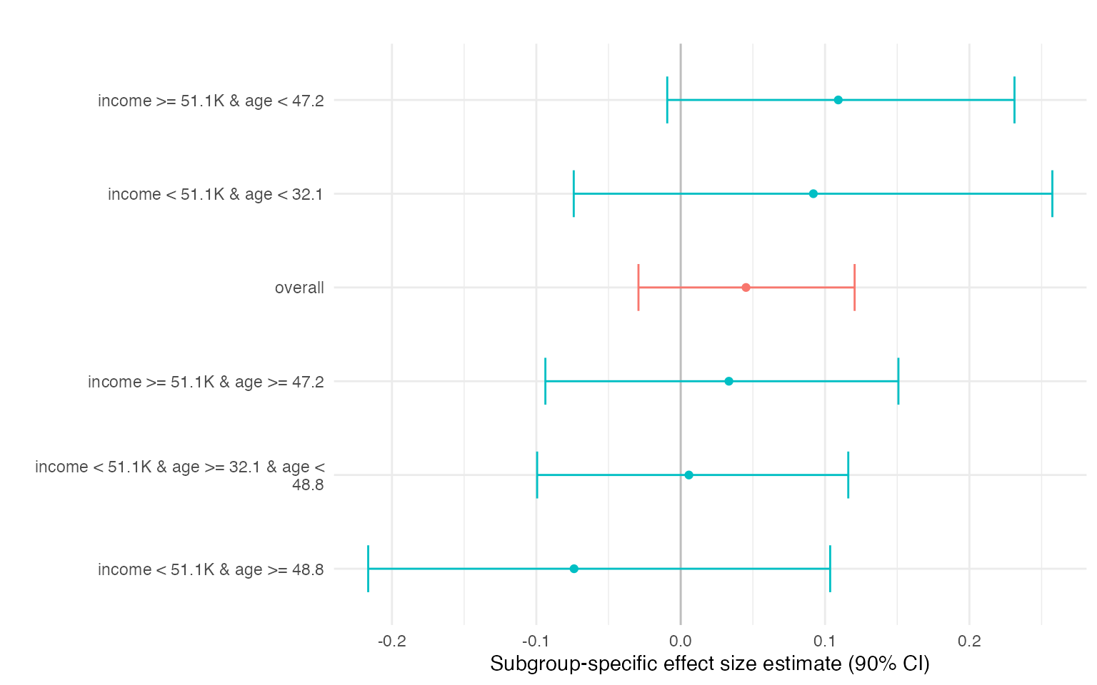
We can automatically find segments (subgroups) with different conditional complier effects using a shallow regression tree on posterior mean CATE_C(x). The segment-level summaries in res$effects correspond to subgroup-specific average effects among compliers, obtained by averaging conditional effects within each covariate-defined segment. Differences across segments highlight departures from effect homogeneity and provide an interpretable summary of treatment effect heterogeneity.

res <- segment_heterogeneity(
  fit,
  min_compliers_bucket = 50,
  plot = TRUE,
  contrast = TRUE
)

res$contrast$summary
#>        mean        sd    ci_lower ci_upper p_gt0
#> 1 0.1830328 0.1233037 -0.03709192 0.379174  0.93
res$plot$diff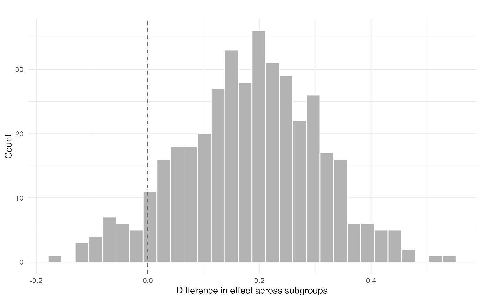

The segment-level summaries in res$effects correspond to subgroup-specific average effects among compliers, obtained by averaging conditional effects within each covariate-defined segment. Differences across segments highlight departures from effect homogeneity and provide an interpretable summary of treatment effect heterogeneity. Segments are constructed post hoc to summarize heterogeneity in the posterior distribution of CATE_C(x).

res$effects
#>                                    segment     mean     sd ci_lower ci_upper
#>                                    overall  0.04523 0.0457 -0.02925    0.120
#>               income < 51.1K & age >= 48.8 -0.07388 0.0956 -0.21647    0.104
#>  income < 51.1K & age >= 32.1 & age < 48.8  0.00568 0.0633 -0.09944    0.116
#>                income < 51.1K & age < 32.1  0.09191 0.1041 -0.07409    0.257
#>              income >= 51.1K & age >= 47.2  0.03339 0.0753 -0.09374    0.151
#>               income >= 51.1K & age < 47.2  0.10916 0.0709 -0.00932    0.231
#>  p_gt0   n n_group
#>  0.833 800   551.3
#>  0.215  68    53.5
#>  0.520 266   191.3
#>  0.815  88    61.3
#>  0.667  83    60.6
#>  0.920 295   184.5
res$plot$effect