FPET: Local fitting for national estimation for all women

Introduction

In this vignette we obtain national estimates of FP indicators for all women. We use local fits.

library(fpet2)
options(cmdstanr_warn_inits = FALSE)

Read data for all countries

We use the Track20 survey data base and the UNPD population estimates:

data_folder <- here::here("data-raw")
survey_data_file <- file.path(data_folder, "Track20 2025 Database for FPET2 051325.csv")
nat_population_data_file <- file.path(data_folder, "population_counts.rds")
# read inputs
survey_df_all <- readr::read_csv(survey_data_file, show_col_types = FALSE)
population_df_all <- readRDS(nat_population_data_file)

Model fitting

First choose a country (division_numeric_code and country names are available in fpet2::regions_all):

division_numeric_code_select <- 768 # Togo

Note that in the current package, the model needs to be compiled once, this takes a little while. (Note: In the 2024 version, we packaged up the model using instantiate, we can consider that again here too).

There will be text indicating what model assumptions are made for married women, followed by assumptions for unmarried women.

results_national <- fit_fpem(
  survey_df = survey_df_all |>
    dplyr::filter(division_numeric_code == division_numeric_code_select),
  population_df = population_df_all |>
    dplyr::filter(division_numeric_code == division_numeric_code_select),
  service_statistic_df = NULL,
  subnational = FALSE,
  regions_dat = fpet2::regions_all
)

## [1] "This is the FPET2025 version 1.2 (released November 24, 2025)!"
## [1] "When imputing SEs for DHS, we use the effective sample size of its preceding survey"

## Joining with `by = join_by(record_id_fixed)`
## Joining with `by = join_by(record_id_fixed)`

## [1] "We define possible outliers based on column possible_outlier"
## [1] "We use a global fit, and take selected settings from there."
## [1] "settings for the spline_degree and num_knots taken from global run"
## [1] "Setting for tstar taken from global run"
## [1] "We take all hier terms from the global fit, using prefix"
## [1] "For hierarchical terms, we fix things up to the 2nd-lowest level."
## [1] "We fix all sigmas of hierarchical models for demand and ds."
## [1] "We take all hier terms from the global fit, using prefix"
## [1] "For hierarchical terms, we fix things up to the 2nd-lowest level."
## [1] "We fix all sigmas of hierarchical models for demand and ds."
## [1] "Local run, we only use data for TGO"
## [1] "We take all hier terms from the global fit, using prefix"
## [1] "For hierarchical terms, we fix things up to the 2nd-lowest level."
## [1] "We fix all sigmas of hierarchical models."
## [1] "When imputing SEs for DHS, we use the effective sample size of its preceding survey"

## Joining with `by = join_by(record_id_fixed)`
## Joining with `by = join_by(record_id_fixed)`

## [1] "We define possible outliers based on column possible_outlier"
## [1] "We use a global fit, and take selected settings from there."
## [1] "settings for the spline_degree and num_knots taken from global run"
## [1] "Setting for tstar taken from global run"
## [1] "We take all hier terms from the global fit, using prefix"
## [1] "For hierarchical terms, we fix things up to the 2nd-lowest level."
## [1] "We fix all sigmas of hierarchical models for demand and ds."
## [1] "We take all hier terms from the global fit, using prefix"
## [1] "For hierarchical terms, we fix things up to the 2nd-lowest level."
## [1] "We fix all sigmas of hierarchical models for demand and ds."
## [1] "Local run, we only use data for TGO"
## [1] "We take all hier terms from the global fit, using prefix"
## [1] "For hierarchical terms, we fix things up to the 2nd-lowest level."
## [1] "We fix all sigmas of hierarchical models."

## Running MCMC with 4 parallel chains...
## 
## Chain 1 Iteration:   1 / 350 [  0%]  (Warmup) 
## Chain 2 Iteration:   1 / 350 [  0%]  (Warmup) 
## Chain 3 Iteration:   1 / 350 [  0%]  (Warmup) 
## Chain 4 Iteration:   1 / 350 [  0%]  (Warmup) 
## Chain 2 Iteration:  50 / 350 [ 14%]  (Warmup) 
## Chain 3 Iteration:  50 / 350 [ 14%]  (Warmup) 
## Chain 1 Iteration:  50 / 350 [ 14%]  (Warmup) 
## Chain 4 Iteration:  50 / 350 [ 14%]  (Warmup) 
## Chain 2 Iteration: 100 / 350 [ 28%]  (Warmup) 
## Chain 3 Iteration: 100 / 350 [ 28%]  (Warmup) 
## Chain 1 Iteration: 100 / 350 [ 28%]  (Warmup) 
## Chain 2 Iteration: 150 / 350 [ 42%]  (Warmup) 
## Chain 2 Iteration: 151 / 350 [ 43%]  (Sampling) 
## Chain 3 Iteration: 150 / 350 [ 42%]  (Warmup) 
## Chain 3 Iteration: 151 / 350 [ 43%]  (Sampling) 
## Chain 4 Iteration: 100 / 350 [ 28%]  (Warmup) 
## Chain 1 Iteration: 150 / 350 [ 42%]  (Warmup) 
## Chain 1 Iteration: 151 / 350 [ 43%]  (Sampling) 
## Chain 2 Iteration: 200 / 350 [ 57%]  (Sampling) 
## Chain 3 Iteration: 200 / 350 [ 57%]  (Sampling) 
## Chain 4 Iteration: 150 / 350 [ 42%]  (Warmup) 
## Chain 4 Iteration: 151 / 350 [ 43%]  (Sampling) 
## Chain 1 Iteration: 200 / 350 [ 57%]  (Sampling) 
## Chain 2 Iteration: 250 / 350 [ 71%]  (Sampling) 
## Chain 3 Iteration: 250 / 350 [ 71%]  (Sampling) 
## Chain 1 Iteration: 250 / 350 [ 71%]  (Sampling) 
## Chain 4 Iteration: 200 / 350 [ 57%]  (Sampling) 
## Chain 2 Iteration: 300 / 350 [ 85%]  (Sampling) 
## Chain 3 Iteration: 300 / 350 [ 85%]  (Sampling) 
## Chain 1 Iteration: 300 / 350 [ 85%]  (Sampling) 
## Chain 4 Iteration: 250 / 350 [ 71%]  (Sampling) 
## Chain 2 Iteration: 350 / 350 [100%]  (Sampling) 
## Chain 2 finished in 7.7 seconds.
## Chain 3 Iteration: 350 / 350 [100%]  (Sampling) 
## Chain 3 finished in 7.9 seconds.
## Chain 1 Iteration: 350 / 350 [100%]  (Sampling) 
## Chain 1 finished in 8.1 seconds.
## Chain 4 Iteration: 300 / 350 [ 85%]  (Sampling) 
## Chain 4 Iteration: 350 / 350 [100%]  (Sampling) 
## Chain 4 finished in 8.7 seconds.
## 
## All 4 chains finished successfully.
## Mean chain execution time: 8.1 seconds.
## Total execution time: 8.8 seconds.
## 
## [1] "Chains finished, now calculating estimates (can take a little while)"

## Joining with `by = join_by(year, marital_status)`

Let’s plot!

plots_all <- plot_estimates_local_all(
  results = results_national,
  subnational  = FALSE,
  dat_emu = results_national$dat_emu,
  save_plots = FALSE)
print(plots_all)

## $TGO
## $TGO$married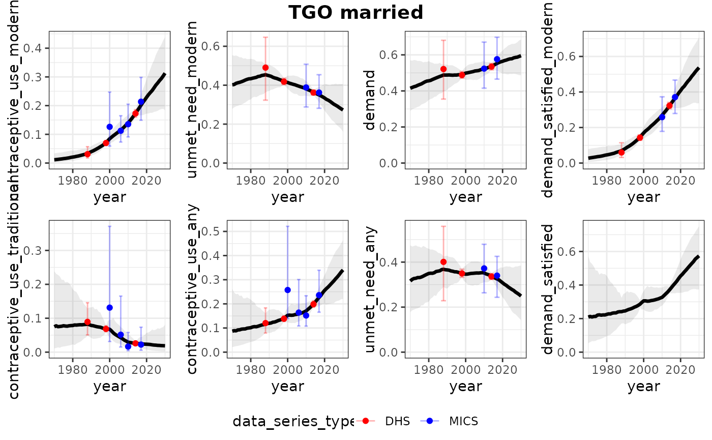

## 
## $TGO$unmarried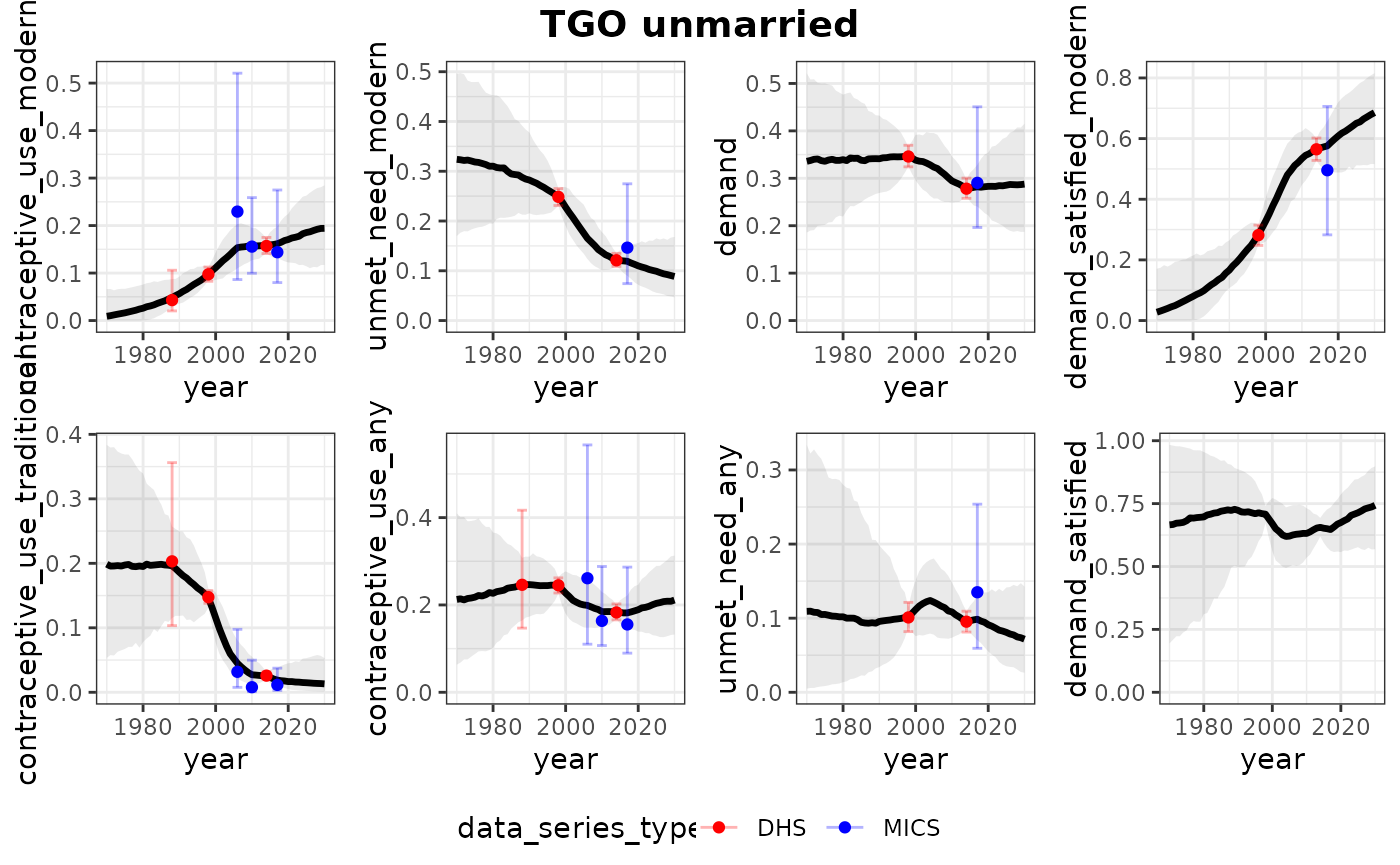

## 
## $TGO$all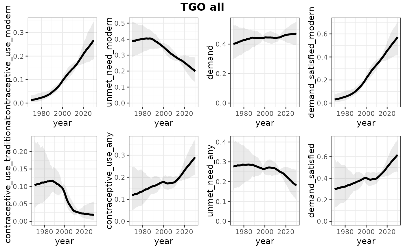

The model fit object also contains the estimates, which can be used for custom plotting or tables. Some examples:

results_national$estimates |>
  dplyr::filter(marital_status == "all")

## # A tibble: 11,712 × 9
##    iso    year indicator         marital_status percentile division_numeric_code
##    <chr> <dbl> <chr>             <chr>          <chr>                      <dbl>
##  1 TGO    1970 contraceptive_us… all            mean                         768
##  2 TGO    1970 contraceptive_us… all            mean                         768
##  3 TGO    1970 contraceptive_us… all            2.5%                         768
##  4 TGO    1970 contraceptive_us… all            2.5%                         768
##  5 TGO    1970 contraceptive_us… all            5%                           768
##  6 TGO    1970 contraceptive_us… all            5%                           768
##  7 TGO    1970 contraceptive_us… all            10%                          768
##  8 TGO    1970 contraceptive_us… all            10%                          768
##  9 TGO    1970 contraceptive_us… all            50%                          768
## 10 TGO    1970 contraceptive_us… all            50%                          768
## # ℹ 11,702 more rows
## # ℹ 3 more variables: region_code <lgl>, measure <chr>, value <dbl>

results_national$estimates |>
  dplyr::filter(measure == "population_count")

## # A tibble: 17,568 × 9
##    iso    year indicator         marital_status percentile division_numeric_code
##    <chr> <dbl> <chr>             <chr>          <chr>                      <dbl>
##  1 TGO    1970 contraceptive_us… married        mean                         768
##  2 TGO    1970 contraceptive_us… married        2.5%                         768
##  3 TGO    1970 contraceptive_us… married        5%                           768
##  4 TGO    1970 contraceptive_us… married        10%                          768
##  5 TGO    1970 contraceptive_us… married        50%                          768
##  6 TGO    1970 contraceptive_us… married        90%                          768
##  7 TGO    1970 contraceptive_us… married        95%                          768
##  8 TGO    1970 contraceptive_us… married        97.5%                        768
##  9 TGO    1970 contraceptive_us… married        mean                         768
## 10 TGO    1970 contraceptive_us… married        2.5%                         768
## # ℹ 17,558 more rows
## # ℹ 3 more variables: region_code <lgl>, measure <chr>, value <dbl>

Leontine Alkema

2025-11-25

Introduction

Read data for all countries

Model fitting